Home

!pip install tensorflow tensorflow_datasets

The above code installs the core libraries needed to build and train machine learning models using TensorFlow and to access ready-to-use datasets. tensorflow is a powerful open-source framework developed by Google for building deep learning models, while tensorflow_datasets provides a wide variety of preprocessed datasets, like the AG News dataset used in this project. The exclamation mark (!) allows this command to be run directly in Jupyter or Colab notebooks as a shell command, making setup quick and seamless.

import tensorflow as tf
import tensorflow_datasets as tfds
from tensorflow.keras.layers import TextVectorization, Embedding, GlobalAveragePooling1D, Dense
from tensorflow.keras.models import Sequential
import matplotlib.pyplot as plt
import gradio as gr

This block imports all the essential libraries used throughout the project. tensorflow as tf loads the TensorFlow library, which provides tools to build and train neural networks. tensorflow_datasets as tfds gives access to a wide range of prebuilt datasets, including AG News, in a ready-to-use format. From tensorflow.keras.layers, we import layers like TextVectorization (to convert text into numbers), Embedding (to map words into dense vectors), GlobalAveragePooling1D (to reduce sequence dimension), and Dense (for fully connected layers). Sequential is imported from tensorflow.keras.models to help us build a layer-by-layer model. matplotlib.pyplot is imported as plt for visualizing training performance like accuracy over epochs. Lastly, gradio as gr brings in Gradio, a library used to create a simple web interface for our trained model so users can interact with it easily.

(train_data, test_data), info = tfds.load(
    'ag_news_subset',
    split=['train[:80%]', 'train[80%:]'],
    as_supervised=True,
    with_info=True
)

This line loads the AG News dataset using tensorflow_datasets and splits it into training and testing subsets. The tfds.load() function downloads the dataset if it’s not already present and returns it in a format ready for use in TensorFlow. The parameter 'ag_news_subset' specifies the dataset name. The split=['train[:80%]', 'train[80%:]'] argument divides the dataset into two parts — the first 80% for training and the remaining 20% for testing — based on the original training set. Setting as_supervised=True returns the data as (text, label) pairs, which is ideal for supervised learning tasks. The with_info=True argument returns a second object, info, containing metadata like the number of classes, labels, and dataset description, which is useful for debugging or display purposes.

VOCAB_SIZE = 10000       # Number of unique words
SEQUENCE_LENGTH = 200    # Max tokens per input
BATCH_SIZE = 32
CLASS_NAMES = ['World', 'Sports', 'Business', 'Sci/Tech']

This section defines a few key constants that shape how the model processes text data. VOCAB_SIZE = 10,000 sets the maximum number of unique words (tokens) the model will recognize, ensuring we focus on the most frequent terms in the dataset. SEQUENCE_LENGTH = 200 limits each input text to 200 tokens, either truncating longer texts or padding shorter ones to maintain uniform input size for the model. BATCH_SIZE = 32 determines how many samples will be processed together during training, balancing speed and memory efficiency. Lastly, CLASS_NAMES is a list that maps numerical prediction outputs (0 to 3) to human-readable category names — World, Sports, Business, and Sci/Tech — making the model’s output easier to interpret.

vectorizer = TextVectorization(max_tokens=VOCAB_SIZE, output_sequence_length=SEQUENCE_LENGTH)
vectorizer.adapt(train_data.map(lambda text, label: text))

This block creates and trains a TextVectorization layer, which transforms raw text into sequences of integers that a neural network can process. The first line initializes the layer with two key parameters: max_tokens=VOCAB_SIZE ensures only the 10,000 most common words are included in the vocabulary, while output_sequence_length=SEQUENCE_LENGTH standardizes the length of each text input to 200 tokens (padding or truncating as needed). The second line prepares the vectorizer by “adapting” it to the dataset — using train_data.map(lambda text, label: text) extracts only the text portion from each (text, label) pair and feeds it into the vectorizer. This lets the layer learn the vocabulary from the training data, effectively mapping each word to a unique integer ID based on its frequency.

def preprocess(text, label):
    return vectorizer(text), label

train_ds = train_data.map(preprocess).cache().shuffle(1000).batch(BATCH_SIZE).prefetch(tf.data.AUTOTUNE)
test_ds = test_data.map(preprocess).batch(BATCH_SIZE).prefetch(tf.data.AUTOTUNE)

This section defines a preprocessing function and prepares the training and testing datasets for efficient feeding into the model. The preprocess function takes a (text, label) pair and returns the text as a vectorized sequence of integers using the TextVectorization layer, while leaving the label unchanged. Next, train_data.map(preprocess) applies this transformation to every example in the training set. The .cache() method stores the dataset in memory after the first epoch, improving performance. .shuffle(1000) randomly mixes 1,000 examples at a time, helping the model generalize better by avoiding patterns in the input order. .batch(BATCH_SIZE) groups data into batches of 32 samples, and .prefetch(tf.data.AUTOTUNE) ensures that while the model is training on one batch, the next is prepared in the background — reducing latency. The test_ds pipeline is similar but excludes shuffling and caching, as evaluation doesn’t require randomness or memory optimization.

model = Sequential([
    Embedding(input_dim=VOCAB_SIZE, output_dim=64),
    GlobalAveragePooling1D(),
    Dense(64, activation='relu'),
    Dense(4, activation='softmax')
])

This block defines the architecture of the neural network using TensorFlow’s Sequential model, which stacks layers in a linear order. The first layer, Embedding(input_dim=VOCAB_SIZE, output_dim=64), creates a 64-dimensional vector representation for each word index — allowing the model to learn semantic relationships between words during training. Next, GlobalAveragePooling1D() compresses the entire sequence of word embeddings into a single fixed-size vector by averaging across all time steps, simplifying the model while preserving the overall context. The Dense(64, activation='relu') layer is a fully connected layer with 64 neurons using the ReLU activation function, which introduces non-linearity and helps the network learn complex patterns. Finally, Dense(4, activation='softmax') is the output layer with 4 neurons — one for each news category — using softmax to convert the output into a probability distribution over the four classes.

model.compile(
    loss='sparse_categorical_crossentropy',
    optimizer='adam',
    metrics=['accuracy']
)
history = model.fit(train_ds, validation_data=test_ds, epochs=5)

This block compiles and trains the model. The model.compile() method sets the configuration for learning. Here, loss='sparse_categorical_crossentropy' is used because the target labels are integers (0 to 3) rather than one-hot encoded vectors — it calculates how far the model’s predicted probability distribution is from the true class. The optimizer='adam' is a popular and efficient choice that adapts the learning rate during training for faster convergence. The model is also set to track 'accuracy' as a metric to evaluate performance during and after training. Next, model.fit() starts the training process. It uses train_ds as the training data, test_ds as validation data (to monitor how well the model generalizes), and trains the model for 5 epochs (full passes through the training dataset). The returned history object stores metrics like loss and accuracy over each epoch, which can later be plotted to visualize the learning progress.

loss, accuracy = model.evaluate(test_ds)
print(f"Test Accuracy: {accuracy * 100:.2f}%")

After training, this block evaluates the model’s performance on the test dataset. The model.evaluate(test_ds) function runs the model on the unseen test_ds data and returns the loss and accuracy metrics. This helps assess how well the model generalizes to new data it hasn’t seen during training. The returned accuracy is a float between 0 and 1, representing the percentage of correct predictions. The print() statement formats and displays this accuracy as a percentage with two decimal places — for example, Test Accuracy: 89.65% — giving a clear summary of the model’s effectiveness on real-world inputs.

plt.plot(history.history['accuracy'], label='Train Accuracy')
plt.plot(history.history['val_accuracy'], label='Validation Accuracy')
plt.xlabel('Epoch')
plt.ylabel('Accuracy')
plt.legend()
plt.title('Accuracy over Epochs')
plt.show()

This block uses Matplotlib to visualize how the model’s accuracy changed during training. The history.history dictionary contains training metrics collected over each epoch. plt.plot(history.history['accuracy'], label='Train Accuracy') plots the accuracy on the training dataset, while plt.plot(history.history['val_accuracy'], label='Validation Accuracy') plots the accuracy on the validation (test) dataset. Adding plt.xlabel('Epoch') and plt.ylabel('Accuracy') labels the axes for clarity. The plt.legend() adds a legend so viewers can distinguish between the two curves. plt.title('Accuracy over Epochs') gives the chart a meaningful title, and finally, plt.show() renders the plot. This visualization helps you see if the model is improving over time, and whether it’s overfitting or underfitting based on the gap between training and validation curves.

def predict_category(text):
    vector = vectorizer([text])
    prediction = model.predict(vector)
    class_id = tf.argmax(prediction[0]).numpy()
    return CLASS_NAMES[class_id]

This function allows us to make predictions on new, unseen text using the trained model. It takes a single text input as a string. First, vectorizer([text]) converts the raw input into a numerical sequence using the same vocabulary and preprocessing as during training. Then, model.predict(vector) passes the processed input through the model and returns a probability distribution over the four classes. The line tf.argmax(prediction[0]) identifies the index of the highest probability — i.e., the most likely category. Finally, CLASS_NAMES[class_id] maps that numeric class ID (0 to 3) back to a human-readable label like "World" or "Sports" and returns it. This function makes it easy to classify any news headline or short article instantly.

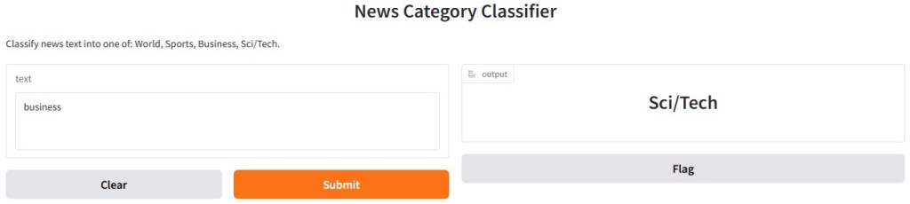
interface = gr.Interface(
    fn=predict_category,
    inputs=gr.Textbox(lines=3, placeholder="Enter a news headline or short article..."),
    outputs=gr.Label(num_top_classes=4),
    title="News Category Classifier",
    description="Classify news text into one of: World, Sports, Business, Sci/Tech."
)
interface.launch()

This block creates a simple, interactive web interface using Gradio, allowing anyone to use the trained model directly in a browser. The gr.Interface() function wraps the predict_category function so users can input text and receive a predicted news category. The inputs=gr.Textbox(...) creates a multiline text box for entering a news headline or short article, with a placeholder to guide the user. The outputs=gr.Label(num_top_classes=4) displays the predicted category and shows the top 4 class probabilities for better insight. The title and description provide context at the top of the interface. Finally, interface.launch() runs a local web server and opens the app in your browser — perfect for demos, testing, or sharing with others.